During this lab, I worked with the IMU.

IMU Setup

Artemis Connections

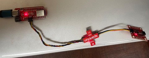
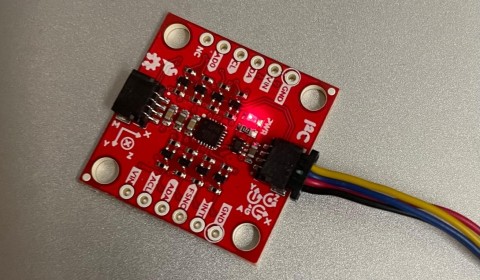
I connected the SparkFun 9DOF IMU to the Artemis Nano via a QWIIC connector.

IMU Sanity Check

After installing the SparkFun 9DOF IMU Breakout_ICM 20948_Arduino Library via Arduino’s library manager, I ran the basic example to verify that the setup was working correctly. You should see something like below,

Scaled. Acc (mg) [  00254.88,  00059.08,  00973.14 ], Gyr (DPS) [ -00001.78, -00000.51, -00001.42 ], Mag (uT) [ -00021.45, -00027.90,  00062.55 ], Tmp (C) [  00034.21 ]

AD0_VAL

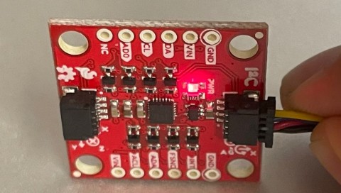
The AD0_VAL refers to the last bit of the I2C address of the IMU. It is by default set to 1 on the IMU, and thus ADO_VAL should be set to 1 to communicate. This value can be changed by closing the ADR jumper which sets it to 0. Also, the IMU seems to offer a AD0 pin which I think can be set by software when connected to a GPIO pin.

Understanding sensor values

Placing the IMU flat on a surface,

The accelerometer and gyro data should look something like

Scaled. Acc (mg) [ -00003.42, -00012.21,  01021.00 ], Gyr (DPS) [ -00001.12,  00001.79,  00000.08 ]

You can see that there is roughly 1g of acceleration due to gravity on the Z-axis.

Placing the IMU on its side as below, you should now see 1g on the y-axis.

The gyro measures the angular velocity of the IMU in degrees per second (DPS). Rotating it around the Z-axis, the angular velocity about the z-axis will increase.

Accelerometer

The accelerometer data can be used to compute the pitch and roll of the IMU via the following formulae, \(p = \text{atan2}(a_z, a_z), r = \text{atan2}(a_x, a_z)\)

Then,

I found that the accelerometer was fairly accurate within about 0.02 rad of the true answer. For 90 degrees pitch, I got 1.58 rad (the true value is 1.57). I got -1.56 for -90 degree pitch. For 90 and -90 roll, I got 1.56 and -1.56 respectively.

Noise in frequency spectrum

While the noise in my testing was fairly low, when running the RC car, there will be a lot of vibrational noise that will make readings noisy. To elimate this, I use a low pass filter.

Fourier Transform

To figure out which frequencies to keep, I obtained timestamped sensor readings from the IMU while I moved it around.

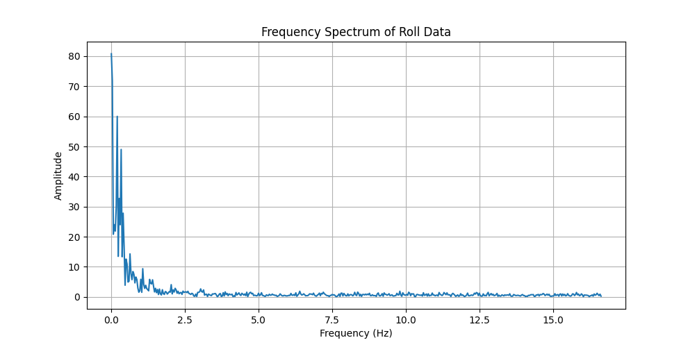
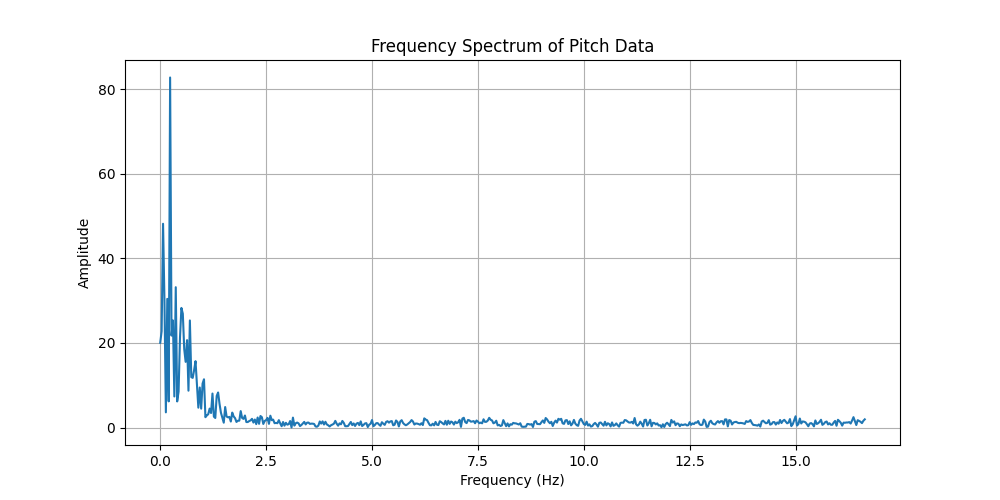
The graphs above show a peak around 0 Hz which is expected, and it shows that the pertinent signal has frequencies > 1.5 Hz. So, eliminating these frequencies should help combat sensor noise.

Low Pass Filter

Using a low pass filter, that’s defined by the following recursive relation, \(y' = \alpha * x + (1-\alpha) * y\) where \(x\) is the raw measurement, \(y\) is the previous filtered measurement and \(y'\) is the new one. Then, to eliminate frequencies greater than \(f_c = 1.5\), set \(\alpha = \frac{1}{1 + \frac{f_s}{2\pi f_c}}\) where \(f_c, f_s\) are the cutoff and sampling frequencies.

Gyroscope

I now use the Gyroscope to obtain roll, pitch and yaw data via dead reckoning. I use the following code for it,

float dt = (float) (times[c] - times[prev])/1000;
float dx = sensor->gyrX()*dt * DEGTORAD;
float dy = sensor->gyrY()*dt * DEGTORAD;
gyr_pitches[c] = gyr_pitches[prev] + dy;
gyr_rolls[c] = gyr_rolls[prev] + dx;
gyr_yaw[c] = gyr_yaw[prev] + sensor->gyrZ()*dt * DEGTORAD;

Using the gyro produces less noisy estimates, but since dead reckoning is used errors accumulate rapidly leading to bias. One can imagine using both measurements in combination to produce a more accurate and less noisy estimat.

Complementary filter

I used a complementary filter to try and get the best of both worlds with the two sensors. I found that the complementary filter was more noisy than just the gyroscopic estimates, but they were less biased.

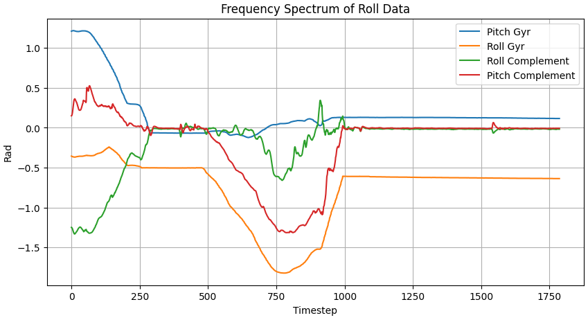The complementary filter is defined as follows,

acc_pitches[c] = lpf(acc_pitches[prev], pitch);
acc_rolls[c] = lpf(acc_rolls[prev], roll);
float dt = (float) (times[c] - times[prev])/1000;
float dx = sensor->gyrX()*dt * DEGTORAD;
float dy = sensor->gyrY()*dt * DEGTORAD;
gyr_pitches[c] = gyr_pitches[prev] + dy;
gyr_rolls[c] = gyr_rolls[prev] + dx;
gyr_yaw[c] = gyr_yaw[prev] + sensor->gyrZ()*dt * DEGTORAD;

comp_pitches[c] = (comp_pitches[prev] + dy)*(1-alpha) +  alpha * acc_pitches[c];
comp_rolls[c] = (comp_rolls[prev] + dx)*(1-alpha) +  alpha * acc_rolls[c];

Sample Data

Speed of Sampling

To improve the sampling speed, I removed all manual delays from the control loop, and every iteration checked whether the sensor data was ready, and if not I continued. During my testing I saw a sample rate of roughly a sample every 2.86 ms which is a rate of 372 samples per second. I created 7 float arrays that stored the filtered pitch, roll from the accelerometer, roll, pitch and yaw from gyro and roll, pitch for the complementary filter. I chose to use floats because the magnitude of the values is not very high, so float precision would suffice. I also had an unsigned int array for timestamps. With a length of 10000 each, it took about 320Kb of memory and can store ~26s of data.

Sending 5s of data over BLE

I used the following code to do this,

void get_data(ICM_20948_I2C *sensor)
{
  times[cnt % ARR_SIZE] = millis();
  float roll = atan2(sensor->accX(), sensor->accZ());
  float pitch = atan2(sensor->accY(), sensor->accZ());
  if (cnt > 0){
    int c = cnt % ARR_SIZE;
    int prev = (cnt - 1) % ARR_SIZE;
    acc_pitches[c] = lpf(acc_pitches[prev], pitch);
    acc_rolls[c] = lpf(acc_rolls[prev], roll);
    float dt = (float) (times[c] - times[prev])/1000;
    float dx = sensor->gyrX()*dt * DEGTORAD;
    float dy = sensor->gyrY()*dt * DEGTORAD;
    gyr_pitches[c] = gyr_pitches[prev] + dy;
    gyr_rolls[c] = gyr_rolls[prev] + dx;
    gyr_yaw[c] = gyr_yaw[prev] + sensor->gyrZ()*dt * DEGTORAD;
    pitches[c] = (pitches[prev] + dy)*(1-alpha) +  alpha * acc_pitches[c];
    rolls[c] = (rolls[prev] + dx)*(1-alpha) +  alpha * acc_rolls[c];
  }
  else{
    acc_pitches[cnt] = pitch;
    acc_rolls[cnt] = roll;
  }
  
}
void loop()
{
  // BLE.advertise();
  BLEDevice central = BLE.central();
    // If a central is connected to the peripheral
  if (central) {
    
      Serial.print("Connected to: ");
      Serial.println(central.address());

      // While central is connected
      while (central.connected()) {
          if (myICM.dataReady()){
            myICM.getAGMT(); 
            // read sensor data
            get_data(&myICM);
          }
          // Read data
          read_data();
          cnt++;
      }

      Serial.println("Disconnected");
  }
}

Stunt

I found the motors had very high torque which allowed the robot flip if you change direction suddenly. The video below demonstrates this

Overall, I learnt a lot about how to combat a lot of the issues like noise and error compounding when using sensors in real life. It was cool to see how well simple exponential moving averages are at smoothing out a signal.